In this tutorial, I use GBS-SNP-CROP to identify variants in a population of tetraploid individuals without a reference genome, starting with the FASTQ files. I then export the allelic read depth to VCF for genotype calling downstream.
Preparing the sequencing data
This section shows how I prepared the data for this tutorial. I did it a little differently from how you might, partly because my lab uses custom adapters and partly because I only wanted to use a few samples in order to create a small dataset that would process quickly. You might instead follow the GBS-SNP-CROP tutorial directly for your own data.
My RAD-seq library was sequenced using single-end reads on a HiSeq 4000, with
inline barcodes (i.e. the barcode is at the beginning of each read, followed
by the remainder of the restriction cut site). There are many tools available
for demultiplexing such data, including
Fastx Toolkit,
Stacks, and
GBS-SNP-CROP. I used my own software
TagDigger because it has the custom
adapters that my lab uses built into it, and will trim them out while performing
the demultiplexing. The CSV passed to the -b argument
lists input file, barcode, and output file for every sample. The argument -a
indicates what adapter set was used. TagDigger and all of the other tools
mentioned generate one FASTQ file for each barcode in the original file, with
the barcode sequence removed.
I ran the code below using Windows Command Prompt, but it would also work in bash.
python barcode_splitter_script.py -b 190419remainingMsa_barcodekey_Hiseq4000.csv -a PstI-MspI-Clark
Out of the files that were generated, we will use the following ones for further analysis. These are all tetraploid, non-hybrid Miscanthus sacchariflorus accessions. If you wish to download the FASTQ files in order to reproduce this entire tutorial, the run accession numbers on NCBI-SRA are provided.
| File | Sample | Provenance | SRA |
|---|---|---|---|
| DOEMsa56a_CCTCCAGA.fq | JM-2014-H-28 | Japan | SRR8997766 |
| DOEMsa56a_CCATAAG.fq | JM-2014-K-8 | Japan | SRR8997767 |
| DOEMsa56a_GGTGGCCA.fq | JM-2014-M-5 | Japan | SRR8997511 |
| DOEMsa56a_GCGGTCCA.fq | JM-2014-S-5 | Japan | SRR8997617 |
| DOEMsa56a_TTGTTGTCTA.fq | JY134 | China | SRR8997716 |
| DOEMsa56a_CCACCATCAG.fq | JY185 | China | SRR8997496 |
| DOEMsa56a_GGTGCCA.fq | KMS257 | South Korea | SRR8997613 |
| DOEMsa56a_TTCTGACA.fq | RU2012-055 | Russia | SRR8991820 |
The sequences then need to all be trimmed to the same length, in particular because the barcodes were variable length and we don’t want to call SNPs at the end of the read where there will be a lot of missing data. We also want to get rid of any low-quality base calls to reduce the number of sequencing errors called as SNPs. Trimmomatic can accomplish this trimming, and we’ll use it here also because it is what is used internally by GBS-SNP-CROP. We will trim the sequences to a maximum of 80 nucleotides, then clip of low-quality sequence at the beginning or end, then discard reads with fewer than 36 nucleotides.
Below is a bash script designed to run on a Linux cluster using Lmod to manage
software. On your own Linux server, you might have to run
java -jar /path/to/trimmomatic-0.38.jar rather than just trimmomatic.
#!/bin/bash

module load Trimmomatic

infiles=("DOEMsa56a_CCTCCAGA.fq" "DOEMsa56a_CCATAAG.fq"
         "DOEMsa56a_GGTGGCCA.fq" "DOEMsa56a_GCGGTCCA.fq"
         "DOEMsa56a_TTGTTGTCTA.fq" "DOEMsa56a_CCACCATCAG.fq"
         "DOEMsa56a_GGTGCCA.fq" "DOEMsa56a_TTCTGACA.fq")
outfiles=("JM-2014-H-28.R1.fq" "JM-2014-K-8.R1.fq"
          "JM-2014-M-5.R1.fq" "JM-2014-S-5.R1.fq"
          "JY134.R1.fq" "JY185.R1.fq" "KMS257.R1.fq" "RU2012-055.R1.fq")

for ((i=0;i<${#infiles[@]};++i)); do
    trimmomatic SE -threads 1 -phred64 ${infiles[i]} ${outfiles[i]} CROP:80 LEADING:3 TRAILING:3 MINLEN:36
done

gzip demultiplexed/*.R1.fq
The gzip line is necessary because GBS-SNP-CROP expects gzipped files.
Assembling the mock reference
We’ll make a tab-delimited text file, that we’ll call Msa_barcodes.txt,
which will indicate the samples in this experiment. The last column with YES
and NO indicates which samples to use for building the mock reference. Two of
the files are smaller than the rest, which is why they are excluded.
CCTCCAGA	JM-2014-H-28	YES
CCATAAG	JM-2014-K-8	YES
GGTGGCCA	JM-2014-M-5	NO
GCGGTCCA	JM-2014-S-5	YES
TTGTTGTCTA	JY134	YES
CCACCATCAG	JY185	NO
GGTGCCA	KMS257	YES
TTCTGACA	RU2012-055	YES
Now we will use GBS-SNP-CROP to build the mock reference.
#!/bin/bash

module load PEAR
module load VSEARCH
module load Perl

perl GBS-SNP-CROP-4.pl -pr pear -vs vsearch -d SE -b Msa_barcodes.txt -t 4 -rl 80 -MR Msa.MR
Again, we are loading pear and vsearch using Lmod, so we can use the program
names directly in place of specifying a path to them. The argument -d SE
incidates that we have single end reads. We will specify four processing cores
using -t 4, and that our reads are 80 nt long using -rl 80. Finally, we
specify the file prefix for our mock reference genome using -MR Msa.MR.
(“Msa” being an abbreviation that the Sacks lab commonly uses for
Miscanthus sacchariflorus.)
Once this is done running, there are some new files in your main directory,
including Msa.MR.Genome.fa, Msa.MR.Clusters.fa, and PosToMask.txt.
We can use less to inspect them.
less Msa.MR.Genome.fa
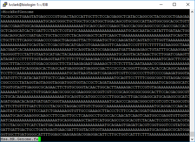
Msa.MR.Genome.fa is what will be used as the reference genome when we align to Msa.
It contains all of the tag clusters separated using strings of A for spacers.
less Msa.MR.Clusters.fa
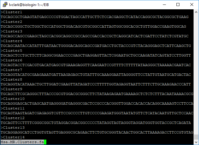
Msa.MR.Clusters.fa isn’t strictly needed for GBS-SNP-CROP, but is there in case
downstream software requires a reference genome.
less PosToMask.txt
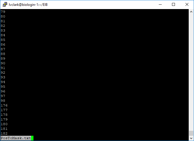
PosToMask.txt contains positions of all spacer nucleotides in Msa.MR.Genome.fa.
Aligning reads to the mock reference and identifying SNPs
The next script in GBS-SNP-CROP uses the alignment software BWA to align every
sequence read to the mock reference that we just created. It then uses SAMtools
to sort and index the alignments, then identify potential SNPs. The -q, -Q,
-f, -F, and -Opt parameters get passed to SAMtools.
#!/bin/bash

module load BWA
module load SAMtools
module load Perl

perl GBS-SNP-CROP-5.pl -bw bwa -st samtools -d SE -b Msa_barcodes.txt -ref Msa.MR.Genome.fa -Q 30 -q 0 -f 0 -F 2308 -t 4 -Opt 0
The most important output from this script is the set of files ending in
.mpileup, which contain information about how reads from each sample correspond
to alleles and loci.
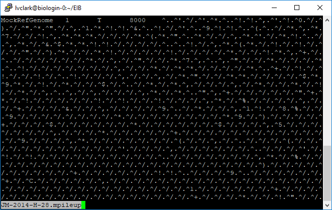
At position 1 in the mock reference, where the reference base is a T, there were 8000 reads that aligned for JM-2014-H-28. The rest of the information is not particularly human-readable, however.
Another script then converts the information from the mpileup files into a
more readable format for further processing. For the sake of having a smaller
dataset to look at in this tutorial, we will only look at SNPs and not indels
(-p snp).
#!/bin/bash

module load Perl

perl GBS-SNP-CROP-6.pl -b Msa_barcodes.txt -out Msa.MasterMatrix.txt -p snp -t 4
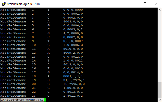
Here we see how many reads corresponded to A, C, G, and T at each position. Scrolling through the file we can see how depth varied from tag to tag.
Additionally, one file was created combining this information from all samples.
Filtering markers
Now we will filter the markers and output them to a genotype matrix. Although GBS-SNP-CROP only makes diploid gentoype calls, which we will not be using, we still want to tweak the parameters so that it can make these calls, because it will throw out SNPs below a given call rate. Here are all the parameters and why I set them as I did:
-mnHoDepth0 20: The default value of5assumes diploidy, where a heterozygote will have alleles in a 1:1 ratio, so the probability of a genotype with five reads having only reads of the first allele is 3%. In tetraploids we will frequently see a 3:1 ratio, so we would need twelve reads to have that same 3% probability. Since we seem to have pretty high depth in this dataset, I increased the number from 12 to 20.-mnHoDepth1 50: When there is just one read of an allele, that read might be due to contamination, or it might indicate a true heterozygote. Again, because we expect heterozygotes that are 3:1 rather than 1:1, we’ll set a higher threshold than the default for determining that a read represents contamination.-mnHetDepth 3: I didn’t see a particular reason to change this from the default. If we see at least three reads, we can start to believe that the allele is really there.-altStrength 0.8: Another one that I kept at the default. If there are multiple alternative alleles, we want most of them to belong to one allele so that GBS-SNP-CROP can convert it to a biallelic marker.-mnAlleleRatio 0.125: This is used for catching paralogous loci that were collapsed into single loci. In a diploid system, we expect a depth ratio of 0.5, but because it can vary due to random chance, the default is to allow it to be as low as 0.25. Since we have a tetraploid and are expecting 0.25, I’ll lower it to 0.125 to allow sampling error. If we see allele depth ratios much below that, it could indicate that a locus isn’t really just one locus.-mnCall 0.75: The default is fine; wanting 75% of samples to have calls for a given SNP is typical.-mnAvgDepth 20: Since we have very high depth, we will set this value higher than the default of3.-mxAvgDepth 3000: Since we have very high depth, we will set this value higher than the default of200.
#!/bin/bash

module load Perl

perl GBS-SNP-CROP-7.pl -in Msa.MasterMatrix.txt -out Msa.GenoMatrix.txt -p snp -mnHoDepth0 20 -mnHoDepth1 50 -mnHetDepth 3 -altStrength 0.8 -mnAlleleRatio 0.125 -mnCall 0.75 -mnAvgDepth 20 -mxAvgDepth 3000
We can see a log of what happened, showing that we got almost 38K SNPs.
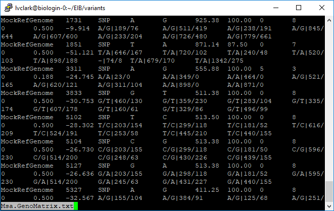
This is what the output genotype matrix looks like. It contains genotype calls and allelic read depth.
Exporting to VCF
Finally, we’ll convert the genotype matrix to a VCF.
#!/bin/bash

module load Perl

perl GBS-SNP-CROP-8.pl -in variants/Msa.GenoMatrix.txt -out Msa_GSCdemo -b Msa_barcodes.txt -formats vcf
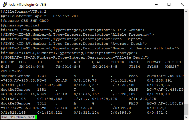
This is the file that we will keep and use for further analysis with other software.